Median House Price Prediction Using Machine Learning

This project demonstrates an end-to-end Machine Learning pipeline to predict median house prices in California using census data. The goal is to provide a reliable, scalable solution for real-estate pricing that outperforms manual estimates.

Project Overview

• Data Collection & Cleaning: Used California census data (1990) and handled missing values.
• Exploratory Analysis & Visualization: Identified correlations and feature distributions.
• Feature Engineering: Created new features (ratios, cluster similarities) and performed transformations (log scaling, standardization).
• Model Training & Selection: Evaluated Linear Regression, Decision Trees, and Random Forests using cross-validation.
• Hyperparameter Tuning: Optimized parameters via GridSearchCV and RandomizedSearchCV.
• Deployment & Monitoring: Saved final model with joblib; emphasized continuous monitoring and retraining.

---

1. Looking at the Big Picture

Before diving into the technical details, let's understand the context of this project. The real estate market is complex, influenced by various factors like location, economic conditions, and demographic trends. Accurate pricing is crucial for buyers, sellers, and investors alike. The task of this project is to build a machine learning model that can predict the median house price in California based on census data(features like population and median income). This model will replace a manual estimation process and feed into a downstream system that helps decide where to invest. Since it's based on labeled data (i.e., known house prices), this is a supervised learning problem.

• Problem Type:
  • Supervised Learning
  • Regression (predicting a continuous value)
  • Multiple Regression (uses many features)
  • Univariate Regression (predicts one value)
  • Batch Learning (data fits in memory and isn’t rapidly changing)
• Performance Metric:
  • Primary: Root Mean Square Error (RMSE) – penalizes large errors more
  • Alternative: Mean Absolute Error (MAE) – less sensitive to outliers
  • Both are norm-based distance measures between predicted and actual values
• Pipeline Design: A data pipeline will handle data transformations step-by-step. Components operate independently and asynchronously, making the system modular and robust but requiring proper monitoring.
• Assumptions Check: Before starting with the technical part, we need to check the assumptions we have: For example the downstream system needs actual price values, not categories. This validates your choice of a regression approach over classification.

Great ! Now we can start with the technical part of the project.

---

2. Get the Data

Starting the technical part of the project by fetching and loading the dataset from an online source. The data is provided as a single compressed file (housing.tgz) containing a CSV file (housing.csv). A Python function is implemented to automate downloading, extracting, and loading the data using Pandas.

Automated Data Retrieval

Data is not accessed from a typical database or multi-file system. Instead, a single function handles:

• Creating the directory (if needed)
• Downloading the file
• Extracting its contents
• Loading the CSV into a DataFrame

Automating this process ensures reproducibility and supports regular updates across multiple machines. Data automation code:

from pathlib import Path
import pandas as pd
import tarfile
import urllib.request

def load_housing_data():
    tarball_path = Path("datasets/housing.tgz")
    if not tarball_path.is_file():
        Path("datasets").mkdir(parents=True, exist_ok=True)
        url = "https://github.com/ageron/data/raw/main/housing.tgz"
        urllib.request.urlretrieve(url, tarball_path)
        with tarfile.open(tarball_path) as housing_tarball:
            housing_tarball.extractall(path="datasets")
    return pd.read_csv(Path("datasets/housing/housing.csv"))

housing = load_housing_data()

Take a Quick Look at the Data

Basic exploration is done before any cleaning or transformation:

• Head(): View the first few rows of the dataset
• Info(): Overview of column types, row count, and missing values
• Describe(): Summary statistics for numerical features

What Was Found – Data Structure:

• Total rows: 20,640
• Features: 10
  • 9 numerical features
  • 1 categorical feature (ocean_proximity)
• Missing data: total_bedrooms has 207 missing values
• median_income is scaled and capped
• median_house_value (target) is capped at $500,000, which may affect predictions
• Histograms show skewed distributions and varying scales

Note: No data cleaning is performed yet — this will be addressed in later sections.

Create a Test Set Early

Before performing any further analysis, a test set must be created and set aside to avoid data snooping bias. Several strategies are discussed:

• Random Sampling: Quick, but may result in unrepresentative samples
• Hash-Based Splitting: Uses unique IDs (e.g., row index or coordinates) to ensure consistent test/train separation across dataset versions
• Stratified Sampling: Ensures key attributes like median_income are proportionally represented using income-based categories

Steps Taken:

• Created income_cat by binning median_income into 5 categories
• Used Scikit-Learn’s StratifiedShuffleSplit to perform stratified sampling
• Dropped the income_cat column after splitting

Key Practice: Creating a test set at the start is a critical part of any machine learning project. It ensures unbiased evaluation and prevents overfitting to the test data during development.

3. Explore and Visualize the Data to Gain Insights

After loading the dataset and setting aside the test set, the next step is to explore the training data more deeply to uncover insights, patterns, and potential issues before moving on to model building.

Initial Setup

Work only with the training set (strat_train_set)

• Make a copy to preserve the original data:

housing = strat_train_set.copy()

Visualizing Geographical Data

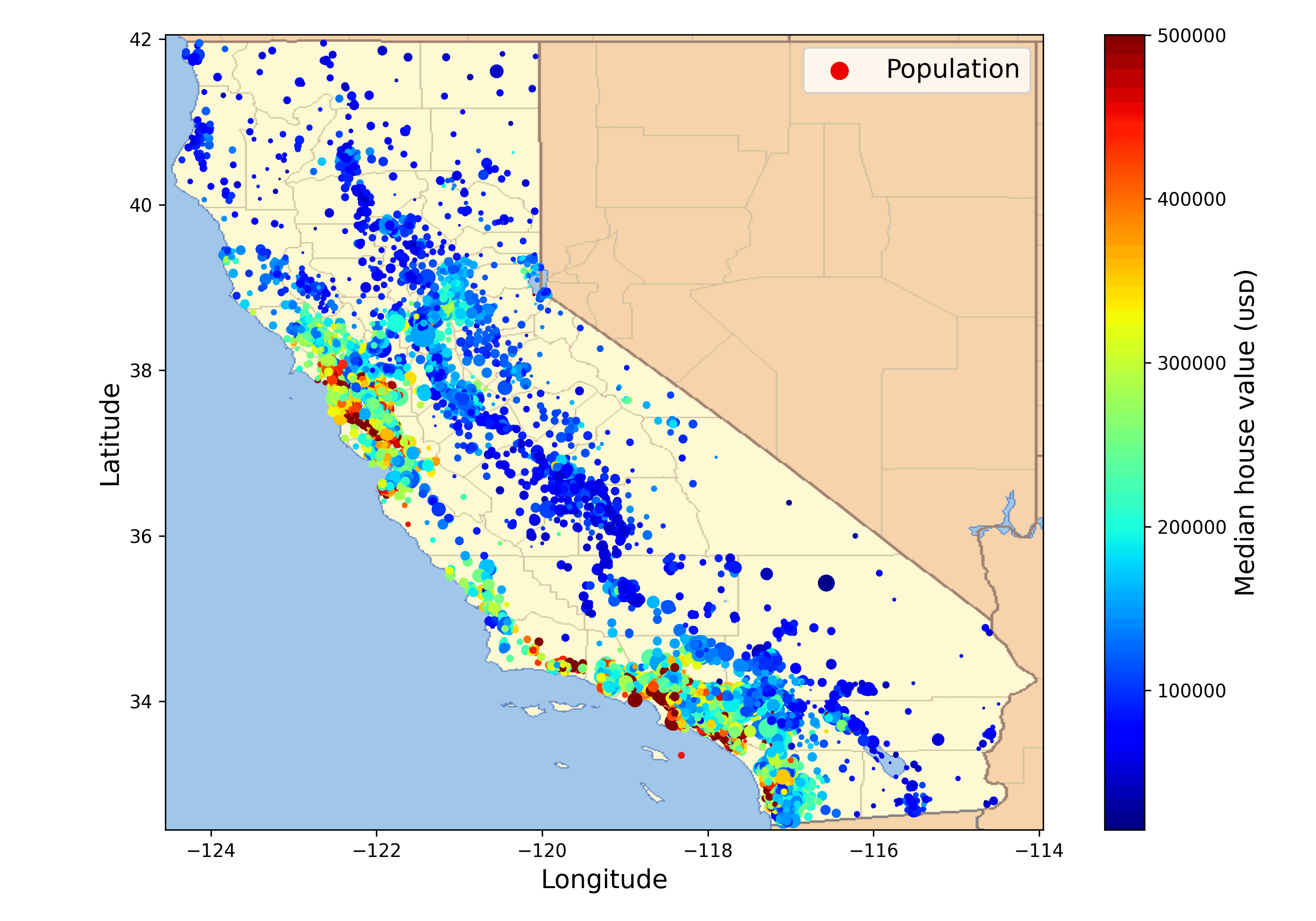
Because the dataset includes geographical information (latitude and longitude), it is a good idea to create a scatterplot of all the districts to visualize the data. Overlay housing prices and population:

housing.plot(kind="scatter", x="longitude", y="latitude", grid=True,
             s=housing["population"] / 100, label="population",
             c="median_house_value", cmap="jet", colorbar=True,
             legend=True, sharex=False, figsize=(10, 7))
plt.show()

• Housing prices correlate with proximity to the coast and high population density.
• High-density clusters observed around San Francisco Bay, Los Angeles, and the Central Valley

Look for Correlations and Create Attribute Combinations

After visualizing the data, the next step is to identify relationships between features and the target (median_house_value). This helps guide feature selection and engineering for your model.

Check for Linear Correlations

using the corr() method to compute the correlation matrix, we can identify which features are most correlated with the target variable (median_house_value).

corr_matrix = housing.corr()
corr_matrix["median_house_value"].sort_values(ascending=False)

Key correlations:

• median_income: Strong positive correlation (0.69) with median_house_value
• total_rooms: Moderate positive correlation (0.14) with median_house_value
• latitude: Moderate negative correlation (-0.14) with median_house_value

Interpretation:

• Values close to 1 or –1 imply strong linear correlation
• Values near 0 indicate little or no linear relationship

Visual Correlation Analysis

using the scatter_matrix() function from Pandas, we can visualize the relationships between features and the target variable. This helps identify potential linear or non-linear relationships.

from pandas.plotting import scatter_matrix

attributes = ["median_house_value", "median_income", "total_rooms",
              "housing_median_age"]
scatter_matrix(housing[attributes], figsize=(12, 8))

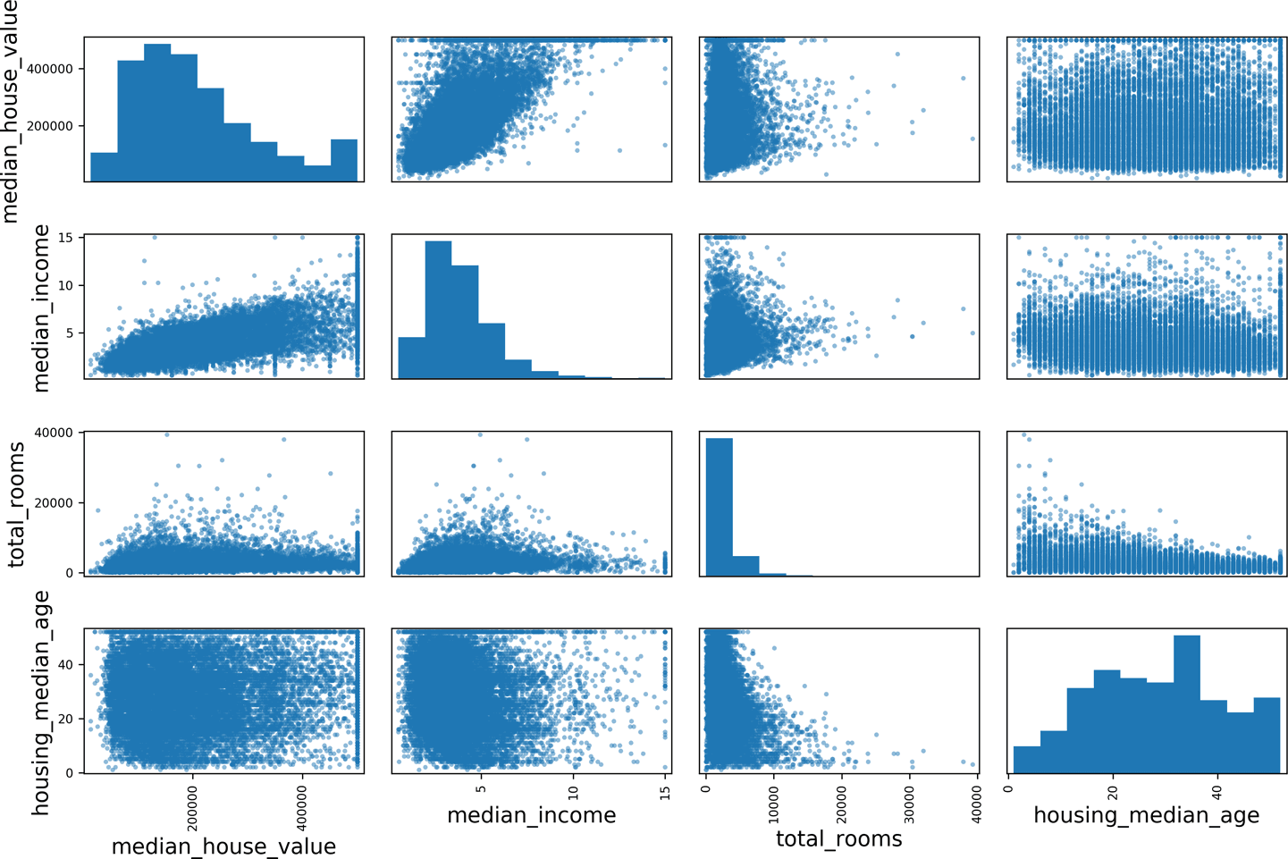
Key observation:

• median_income shows the clearest positive trend with median_house_value, indicating a strong linear relationship.
• Other features like total_rooms and housing_median_age also show some correlation, but less clearly.

Zooming in for detailed inspection:

housing.plot(kind="scatter", x="median_income", y="median_house_value",
             alpha=0.1)

Observations:

• Strong linear trend
• Artificial price cap visible at $500,000 and other flat lines suggest data quirks

Note: Correlation coefficient detects only linear relationships. Nonlinear patterns may still exist even if correlation is near zero.

Engineer New Feature Combinations

Feature combinations often reveal stronger signals than raw attributes. New features created:

housing["rooms_per_house"] = housing["total_rooms"] / housing["households"]
housing["bedrooms_ratio"] = housing["total_bedrooms"] / housing["total_rooms"]
housing["people_per_house"] = housing["population"] / housing["households"]

Updated correlation results:

• bedrooms_ratio: –0.26 (stronger than original bedroom or room counts)
• rooms_per_house: 0.14 (more useful than total_rooms)
• people_per_house: weak negative correlation

---

4. Prepare the Data for Machine Learning Algorithms

Before feeding the data into a model, it must be cleaned and preprocessed. To ensure reproducibility and flexibility, all transformations are done using reusable functions or Scikit-Learn tools.

starting of with a clean copy of the training set:

housing = strat_train_set.drop("median_house_value", axis=1)  # drop labels for training set
housing_labels = strat_train_set["median_house_value"].copy()  # keep labels

Data Cleaning

Handling missing values is crucial for model performance. The total_bedrooms column has 207 missing values, which can be addressed in several ways:

• Drop the rows with missing values
• Drop the attribute entirely
• Fill missing values with a constant (e.g., median)

Use Scikit-Learn’s SimpleImputer with strategy set to "median":

from sklearn.impute import SimpleImputer
imputer = SimpleImputer(strategy="median")
housing_num = housing.drop("ocean_proximity", axis=1)
imputer.fit(housing_num)
X = imputer.transform(housing_num)
housing_tr = pd.DataFrame(X, columns=housing_num.columns, index=housing_num.index)

Handling Text and Categorical Attributes

The ocean_proximity column is categorical. It needs to be converted into a numerical format for the model to understand. Convert it to numbers using:

• OrdinalEncoder: simple encoding but assumes order
• OneHotEncoder: preferred for unordered categories

from sklearn.preprocessing import OneHotEncoder
cat_encoder = OneHotEncoder()
housing_cat_1hot = cat_encoder.fit_transform(housing[["ocean_proximity"]])

Output is a sparse matrix, which saves memory

Custom Transformers

Although Scikit-Learn provides many useful transformers, you will need to write your own for tasks such as custom cleanup operations or combining specific attributes. You will want your transformer to work seamlessly with Scikit-Learn functionalities (such as pipelines), and since Scikit-Learn relies on duck typing (not inheritance), all you need to do is create a class and implement three methods: fit() (returning self), transform(), and fit_transform(). Use BaseEstimator and TransformerMixin to create your own transformer.

from sklearn.base import BaseEstimator, TransformerMixin

class CombinedAttributesAdder(BaseEstimator, TransformerMixin):
    def __init__(self, add_bedrooms_per_room=True):
        self.add_bedrooms_per_room = add_bedrooms_per_room
    def fit(self, X, y=None):
        return self
    def transform(self, X):
        rooms_per_household = X[:, 3] / X[:, 6]
        population_per_household = X[:, 5] / X[:, 6]
        if self.add_bedrooms_per_room:
            bedrooms_per_room = X[:, 4] / X[:, 3]
            return np.c_[X, rooms_per_household, population_per_household, bedrooms_per_room]
        else:
            return np.c_[X, rooms_per_household, population_per_household]

Feature Scaling

Most ML models perform poorly when features have different scales. Two common approaches:

• Min-Max Scaling (0 to 1): MinMaxScaler
• Standardization (mean = 0, std = 1): StandardScaler

from sklearn.preprocessing import StandardScaler
scaler = StandardScaler()
housing_scaled = scaler.fit_transform(housing_num)

Transformation Pipelines#

Using Scikit-Learn’s Pipeline to sequence transformations:

from sklearn.pipeline import Pipeline

num_pipeline = Pipeline([
    ('imputer', SimpleImputer(strategy="median")),
    ('attribs_adder', CombinedAttributesAdder()),
    ('std_scaler', StandardScaler()),
])
housing_num_tr = num_pipeline.fit_transform(housing_num)

Using ColumnTransformer to apply transformations to specific columns:

from sklearn.compose import ColumnTransformer

num_attribs = list(housing_num)
cat_attribs = ["ocean_proximity"]

full_pipeline = ColumnTransformer([
    ("num", num_pipeline, num_attribs),
    ("cat", OneHotEncoder(), cat_attribs),
])

housing_prepared = full_pipeline.fit_transform(housing)

• Handles both numerical and categorical columns
• Outputs a dense or sparse matrix based on matrix density

---

5. Select and Train a Model

With the data fully preprocessed and transformed, the next step is to train and evaluate Machine Learning models. Starting simple, evaluate performance, and gradually experimenting with more complex models using cross-validation.

Train and Evaluate on the Training Set

To begin, a Linear Regression model is trained. This is a simple baseline model that assumes a linear relationship between the input features and the target value (median_house_value).

from sklearn.linear_model import LinearRegression

lin_reg = LinearRegression()
lin_reg.fit(housing_prepared, housing_labels)

The model is then used to predict housing prices for a few instances from the training set:

some_data = housing.iloc[:5]
some_labels = housing_labels.iloc[:5]
some_data_prepared = full_pipeline.transform(some_data)
print("Predictions:", lin_reg.predict(some_data_prepared))
print("Labels:", list(some_labels))

# Predictions: [ 210644.6045  317768.8069  210956.4333  59218.9888  189747.5584]
# Labels: [286600.0, 340600.0, 196900.0, 46300.0, 254500.0]

While the predictions work, they are far from accurate (some predictions differ from actual values by tens of thousands of dollars). To measure how well the model performs overall, the Root Mean Squared Error (RMSE) is used:

from sklearn.metrics import mean_squared_error

housing_predictions = lin_reg.predict(housing_prepared)
lin_mse = mean_squared_error(housing_labels, housing_predictions)
lin_rmse = np.sqrt(lin_mse)
lin_rmse

# 68628.19819848923

Results:

• Linear Regression RMSE ≈ 68,628. This error is quite large considering typical house prices range between $120,000–$265,000.

Interpretation:

• The model is too simple to capture the underlying patterns in the data.

• Solutions include using a more complex model, engineering better features, or reducing constraints (regularization isn’t applied in this case).

Try a More Complex Model – Decision Tree

Next, a Decision Tree Regressor is used. This model is non-linear and capable of learning more complex relationships in the data.

from sklearn.tree import DecisionTreeRegressor

tree_reg = DecisionTreeRegressor()
tree_reg.fit(housing_prepared, housing_labels)

Again, predictions are made and evaluated using RMSE:

housing_predictions = tree_reg.predict(housing_prepared)
tree_mse = mean_squared_error(housing_labels, housing_predictions)
tree_rmse = np.sqrt(tree_mse)

# 0.0

Results:

• Decision Tree RMSE = 0.0 This indicates the model perfectly fits the training data, which is a sign of overfitting. The model is too complex and captures noise rather than the underlying pattern. While it performs perfectly on training data, it is likely to perform poorly on new, unseen data.

Better Evaluation with Cross-Validation

To evaluate models more realistically (without using the test set yet), K-Fold Cross-Validation is used. This technique splits the training set into k folds (e.g., 10), trains the model on k-1 folds, and validates it on the remaining fold—repeating this process k times.

from sklearn.model_selection import cross_val_score

scores = cross_val_score(tree_reg, housing_prepared, housing_labels,
                         scoring="neg_mean_squared_error", cv=10)
tree_rmse_scores = np.sqrt(-scores)

Note: Scikit-Learn uses "negative mean squared error" because it expects a score function (higher is better). That’s why -scores is used.

def display_scores(scores):
    print("Scores:", scores)
    print("Mean:", scores.mean())
    print("Standard deviation:", scores.std())

display_scores(tree_rmse_scores)

# Scores: [70194.33680785 66855.16363941 72432.58244769 70758.73896782
#  71115.88230639 75585.14172901 70262.86139133 70273.6325285
#  75366.87952553 71231.65726027]
# Mean: 71407.68766037929
# Standard deviation: 2439.4345041191004

Results:

• Decision Tree CV RMSE Mean ≈ 71,408
• Standard Deviation ≈ 2,439

Interpretation:

• The Decision Tree overfits the training data and generalizes poorly.
• Cross-validation gives a more realistic view of model performance and helps estimate variance in results.

Compare with Linear Regression (Cross-Validation)

Applying the same cross-validation process to the Linear Regression model:

lin_scores = cross_val_score(lin_reg, housing_prepared, housing_labels,
                             scoring="neg_mean_squared_error", cv=10)
lin_rmse_scores = np.sqrt(-lin_scores)
display_scores(lin_rmse_scores)

# Scores: [66782.73843989 66960.118071   70347.95244419 74739.57052552
#  68031.13388938 71193.84183426 64969.63056405 68281.61137997
#  71552.91566558 67665.10082067]
# Mean: 69052.46136345083
# Standard deviation: 2731.674001798348

Results:

• Linear Regression CV RMSE Mean ≈ 69,052

• Standard Deviation ≈ 2,732

Interpretation:

• Even though Linear Regression underfits the training data, it generalizes better than the overfitting Decision Tree model.

• This underscores the importance of using cross-validation, not just training performance.

Try a More Advanced Model – Random Forest

A Random Forest Regressor is trained next. This ensemble model builds multiple Decision Trees and averages their predictions, reducing overfitting and improving generalization.

from sklearn.ensemble import RandomForestRegressor

forest_reg = RandomForestRegressor()
forest_reg.fit(housing_prepared, housing_labels)

Evaluate using cross-validation:

forest_scores = cross_val_score(forest_reg, housing_prepared, housing_labels,
                                scoring="neg_mean_squared_error", cv=10)
forest_rmse_scores = np.sqrt(-forest_scores)
display_scores(forest_rmse_scores)

Results:

• Random Forest CV RMSE Mean ≈ 50,182

• Standard Deviation ≈ 2,097

• Training RMSE: ~18,603

Interpretation:

• Best performance so far

• Still shows a gap between training and validation scores → some overfitting

• Further improvements may come from:

  • Hyperparameter tuning

  • Feature selection/engineering

  • Using more data

  • Trying other model types (e.g., SVMs, Neural Networks)

Save the Model

It’s good practice to save models and their performance results for later comparison and deployment:

import joblib

joblib.dump(forest_reg, "random_forest_model.pkl")
# Load later
forest_model_loaded = joblib.load("random_forest_model.pkl")

Saved models can store:

• Trained parameters

• Hyperparameters

• Cross-validation scores

• Prediction results

---

6. Fine-Tune The Model

After shortlisting the best-performing models through training and validation, the next step is to fine-tune them to extract maximum performance. This involves adjusting hyperparameters (model configuration settings that aren’t learned during training) to improve accuracy and reduce error.

Option 1: Grid Search (Exhaustive Search)

Grid Search is a brute-force technique where you explicitly define a set of values for each hyperparameter, and Scikit-Learn tests all combinations using cross-validation.

from sklearn.model_selection import GridSearchCV

param_grid = [
    {'n_estimators': [3, 10, 30], 'max_features': [2, 4, 6, 8]},
    {'bootstrap': [False], 'n_estimators': [3, 10], 'max_features': [2, 3, 4]},
]

forest_reg = RandomForestRegressor()

grid_search = GridSearchCV(forest_reg, param_grid, cv=5,
                           scoring='neg_mean_squared_error',
                           return_train_score=True)

grid_search.fit(housing_prepared, housing_labels)

• 18 combinations of hyperparameters
• Each evaluated over 5 folds of data (cross-validation)
• Total of 90 training runs

grid_search.best_params_      # Best parameter combination
grid_search.best_estimator_   # Fully trained model with best parameters
grid_search.best_score_       # Best cross-validation score

Interpretation:

• If the best parameters are at the upper limit (e.g., n_estimators=30), it suggests trying larger values in the next grid.
• You can retrieve all results using grid_search.cv_results_ and sort or visualize them.

Option 2: Randomized Search (Efficient Sampling)

Instead of testing all combinations, RandomizedSearchCV randomly samples a fixed number of combinations from specified ranges or distributions. This is more efficient when:

• The search space is large

• Some hyperparameters have diminishing returns

• You want control over runtime (via number of iterations)

Benefits:

• More variety explored per hyperparameter

• Flexible computational budgeting

Ensemble Methods

Instead of choosing just one model, ensemble learning combines multiple models to improve performance and reduce overfitting.

• Random Forests are an ensemble of Decision Trees

• You can also manually combine the top-performing models

• Ensembles work best when constituent models make different types of errors

More about ensembling techniques (e.g., bagging, boosting, stacking) will be explored in future chapters.

Analyze the Best Model

Feature Importance Random Forests can report the importance of each feature in making predictions. This helps in feature selection and model interpretation.

feature_importances = grid_search.best_estimator_.feature_importances_

You can match these scores to attribute names and sort them:

attributes = num_attribs + extra_attribs + list(cat_encoder.categories_[0])
sorted(zip(feature_importances, attributes), reverse=True)

Takeaway: median_income is by far the most predictive feature. Categorical values like 'ISLAND' are almost useless and may be dropped.

Final Step: Evaluate on the Test Set

After tuning your model with cross-validation, test it once on the held-out test set to estimate real-world performance.

X_test = strat_test_set.drop("median_house_value", axis=1)
y_test = strat_test_set["median_house_value"].copy()

final_predictions = final_model.predict(X_test)

final_rmse = root_mean_squared_error(y_test, final_predictions)
print(final_rmse)  # prints 41424.40026462184

This is lower than previous cross-validation scores, indicating strong generalization.

Confidence Interval for RMSE

To get a range instead of a single score, compute a 95% confidence interval:

from scipy import stats

def rmse(squared_errors):
    return np.sqrt(np.mean(squared_errors))

confidence = 0.95
squared_errors = (final_predictions - y_test) ** 2
boot_result = stats.bootstrap([squared_errors], rmse,
                              confidence_level=confidence, random_state=42)
rmse_lower, rmse_upper = boot_result.confidence_interval  # (39,574 to 43,780)

Interpretation: You can be 95% confident that the true RMSE on new data will fall within this range.

Links

• GitHub code link